LEVITATION

Hello everybody. In this post I'm going to talk about levitation. Levitation is the process by which and object is suspended by a physical force against gravity, in a stable position without solid physical contact. There are a number of different methods that are available in order to levitate a matter, and these methods are:

              1)  Aerodynamic levitation,

        2) Magnetic levitation,

              3) Acoustic levitation,

              4) Quantum levitation,

              5)  Electromagnetic levitation

              6) Electrostatic levitation and

              7)  Optical levitation 

Aerodynamic levitation – is the use of gas pressure to levitate materials so that they are no longer in physical contact with any container. The term aerodynamic levitation could be applied to many objects that use gas pressure to counter the force of gravity, and allow stable levitation. Helicopters and air hockey pucks are two good examples of objects that are aerodynamically levitated. However, more recently this term has also been associated with a scientific technique which uses a cone-shaped nozzle allowing stable levitation of 1-3mm diameter spherical samples without the need for active control mechanisms. 

Magnetic levitation - maglev, or magnetic suspension is a method by which an object is suspended with no support other than magnetic fields. In this case the magnetic pressure is used to counteract the effects of gravitational and any other acceleration. There are two stabilities of magnetically levitated objects and these stabilities are:

-          Static stability means that any small displacement of levitated object from a stable equilibrium position will cause a net force to push it back to the equilibrium point.

-          Dynamic stability occurs when the levitation system is able to damp out any vibration-like motion that may occur.

For successful levitation and control of all 6 axes (3 spatial and 3 rotational) a combination of permanent magnets and electromagnets or diamagnets or superconductors as well as attractive and repulsive fields can be used. From Earnshaw's theorem at least one stable axis must be present for the system to levitate successfully, but the other axes can be stabilized using ferromagnetism.The primary ones used in maglev trains are servo-stabilized electromagnetic suspension (EMS), electrodynamic suspension (EDS).

Acoustic Levitation is a method for suspending matter in a medium by using acoustic radiation pressure from intense sound waves in the medium. Acoustic levitation is possible because of the nonlinear effects of intense sound waves. The objects can be levitated with sound which is heard by the human ear or the sound that levitates object is far from human hearing range.

The first theoretical study was done by L.V.King in 1934 in a paper called “On the Acoustic Radiation Pressure on Spheres”. Unfortunately it was only theoretical because it wasn’t possible to develop the machine that would levitate objects. In 70s and 80s the acoustic levitation was a field of research for NASA and MIT engineers. There is couple of studies available on the internet. In 2013 Swiss scientists made controllable acoustic levitator. So far the levitators could levitate the objects but these hovering objects where motionless. Now they can controllably move these hovering objects. 

 

Acoustic levitation is usually used for containerless processing which has become more important of late due to the small size and resistance of microchips and other such things in industry. Containerless processing may also be used for applications requiring very-high-purity materials or chemical reactions too rigorous to happen in a container. This method is harder to control than other methods of containerless processing such as electromagnetic levitation but has the advantage of being able to levitate nonconducting materials.

Here are couple of videos:

There are many ways of creating this effect, from creating a wave underneath the object and reflecting it back to its source, to using an acrylic glass tank to create a large acoustic field.

Quantum levitation as it is called is a process where scientists use the properties of quantum physics to levitate an object (specifically, a superconductor) over a magnetic source (specifically a quantum levitation track designed for this purpose).

The Science of Quantum Levitation-The reason this works is something called the Meissner effect and magnetic flux pinning. The Meissner effect dictates that a superconductor in a magnetic field will always expel the magnetic field inside of it, and thus bend the magnetic field around it. The problem is a matter of equilibrium. If you just placed a superconductor on top of a magnet, then the superconductor would just float off the magnet, sort of like trying to balance two south magnetic poles of bar magnets against each other.

    Superconductivity and magnetic field do not like each other. When possible, the superconductor will expel all the magnetic field from inside. This is the Meissner effect. In our case, since the superconductor is extremely thin, the magnetic field DOES penetrate. However, it does that in discrete quantities (this is quantum physics after all! ) called flux tubes. (Note: This is demonstrated in the graphic associated with this article.)Inside each magnetic flux tube superconductivity is locally destroyed. The superconductor will try to keep the magnetic tubes pinned in weak areas (e.g. grain boundaries). Any spatial movement of the superconductor will cause the flux tubes to move. In order to prevent that the superconductor remains "trapped" in midair. Let's think about what a superconductor really is: it's a material in which electrons are able to flow very easily. Electrons flow through superconductors with no resistance, so that when magnetic fields get close to a superconducting material, the superconductor forms small currents on its surface, cancelling out the incoming magnetic field. The result is that the magnetic field intensity inside the surface of the superconductor is precisely zero. If you mapped the net magnetic field lines (again, see the graphic) it would show that they're bending around the object. When a superconductor is placed on a magnetic track, the effect is that the superconductor remains above the track, essentially being pushed away by the strong magnetic field right at the track's surface. There is a limit to how far above the track it can be pushed, of course, since the power of the magnetic repulsion has to counteract the force of gravity.

A disk of a type-I superconductor will demonstrate the Meissner effect in its most extreme version, which is called "perfect diamagnetism," and will not contain any magnetic fields inside the material. It'll levitate, as it tries to avoid any contact with the magnetic field. The problem with this is that the levitation isn't stable. The levitating object won't normally stay in place. (This same process has been able to levitate superconductors within a concave, bowl-shaped lead magnet, in which the magnetism is pushing equally on all sides.)One of the key elements of the quantum locking process is the existence of these flux tubes, called a "vortex". If a superconductor is very thin, or if the superconductor is a type-II superconductor, is costs the superconductor less energy to allow some of the magnetic field to penetrate the superconductor. That's why the flux vortices form, in regions where the magnetic field is able to, in effect, "slip through" the superconductor. In the case described by the Tel Aviv team above, they were able to grow a special thin ceramic film over the surface of a wafer. When cooled, this ceramic material is a type-II superconductor. Because it's so thin, the diamagnetism exhibited isn't perfect ... allowing for the creation of these flux vortices passing through the material.

Flux vortices can also form in type-II superconductors, even if the superconductor material isn't quite so thin. The type-II superconductor can be designed to enhance this effect, called "enhanced flux pinning."

Other Types of Quantum Levitation

The process of quantum levitation described above is based on magnetic repulsion, but there are other methods of quantum levitation that have been proposed, including some based on the Casimir effect. Again, this involves some curious manipulation of the electromagnetic properties of the material, so it remains to be seen how practical it is.

The Future of Quantum Levitation

Unfortunately, the current intensity of this effect is such that we won't have flying cars for quite some time. Also, it only works over a strong magnetic field, meaning that we'd need to build new magnetic track roads. However, there are already magnetic levitation trains in Asia which use this process, in addition to the more traditional electromagnetic levitation (maglev) trains. Another useful application is the creation of truly frictionless bearings. The bearing would be able to rotate, but it would be suspended without direct physical contact with the surrounding housing, so that there wouldn't be any friction. There will certainly be some industrial applications for this, and I'll keep my eyes open for when they hit the news.

Electrostatic levitation is the process of using an electric field to levitate a charged object and counteract the effects of gravity. It was used, for instance, in Robert Millikan's oil drop experiment and is used to suspend the gyroscopes in Gravity Probe B during launch.

Due to Earnshaw's theorem no static arrangement of classical electrostatic fields can be used to stably levitate a point charge. There is an equilibrium point where the two fields cancel, but it is an unstable equilibrium. By using feedback techniques it is possible to adjust the charges to achieve a quasi-static levitation.

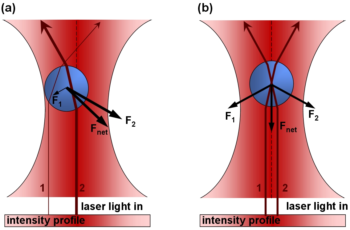
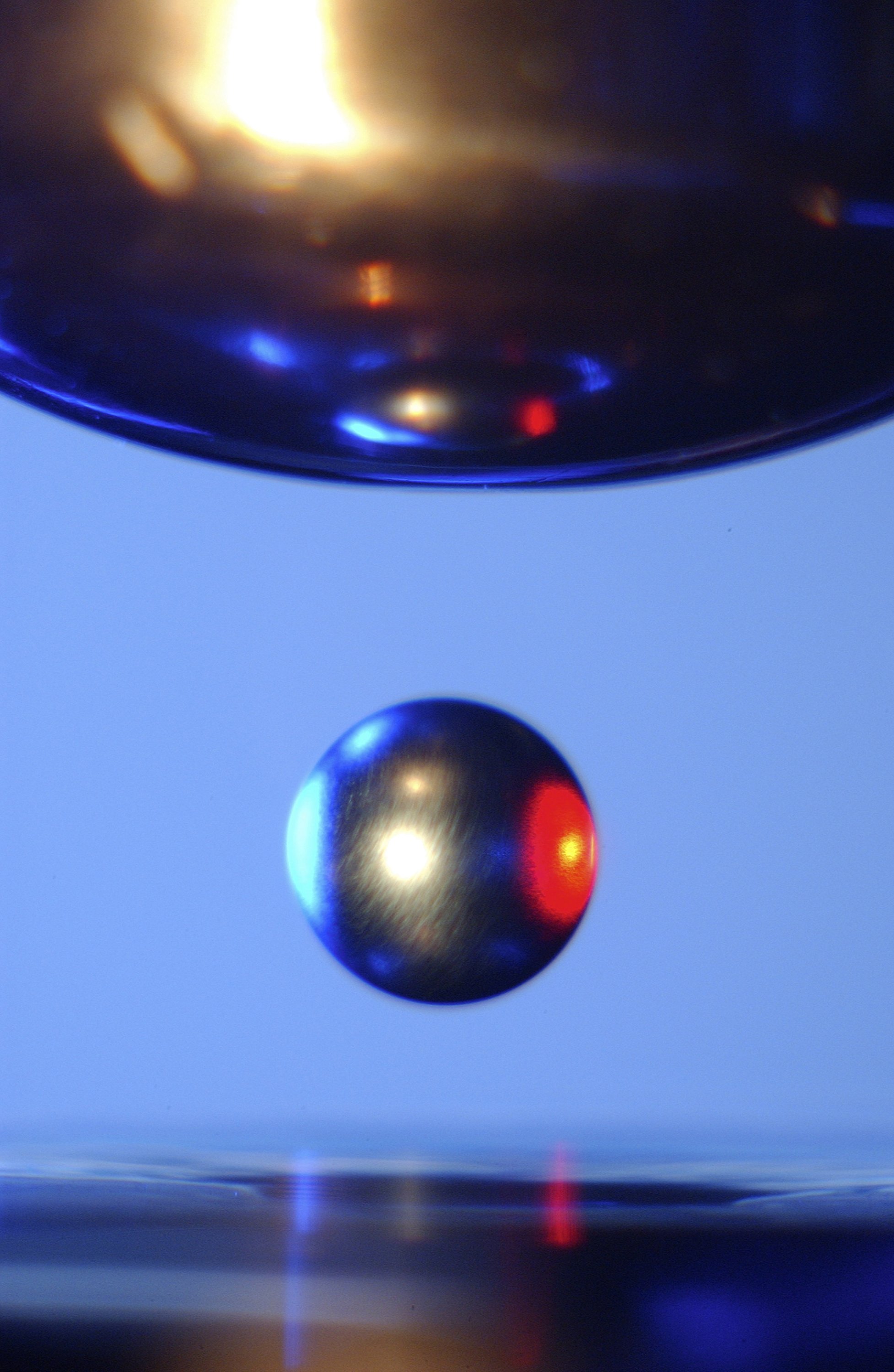
Optical levitation is a method whereby a material is levitates against downward force of gravity by an upward force stemming from photon momentum transfer. Typically photon radiation pressure of a vertical upwardly directed and focused laser beam of enough intensity counters the downward force of gravity to allow for a stable optical trap capable of holding small particles in suspension. 

Specifičnost nelinearnih dinamičkih sustava

Nelinearni dinamički sustavi imaju neka specifična svojstva koja se ne opažaju kod linearnih dinamičkih sustava. Ta svojstva je bitno istaknuti kako bi se dodatno naglasio oprez prilikom nekritične linearizacije nelinearnih dinamičkih sustava. Linearizacijom takvih sustava razaramo navedene osobine sustava, što znači da se linearna aproksimacija može totalno razlikovati u području gdje se dotične osobine ispoljavaju. Navodimo samo one osobine koje se ne mogu pojaviti kod linearnih sustava .

Višestruke fiksne točke. Nelinearni sustavi mogu imati više fiksnih točaka, ili točke ravnoteže. Fiksne ili ravnotežne točke kod nelinearnih autonomnih sustava
$$\dot{x}=f\left( x \right),\text{ }x\left( 0 \right)={{x}_{0}}$$

su oni vektori stanja  za koje je , odnosno koji zadovoljavaju.
$$f\left( {{x}^{*}} \right)=0.$$

Kod linearnih autonomnih sustava postoji samo jedno ravnotežno stanje

Primjer: Jedan jednostavan primjer višestrukih fiksnih točaka je jednadžba slobodnih njihala
$$\ddot{x}+\frac{g}{l}\sin \left( x \right)=0,$$

gdje je x kut njihala od položaja ravnoteže, g je gravitacijska konstanta, a l je duljina njihala. Ravnotežne točke definirane su jednadžbom , čije rješenje je , gdje je n bilo koji prirodni borj. Drugim riječima, imamo beskonačni broj fiksnih točaka.

Konačno vrijeme 'bijega' (finite escape time). Razmotrimo sljedeći nelinearni sustav prvog reda
$$\dot{x}=-x+{{x}^{2}}=0,\text{ }x\left( 0 \right)={{x}_{0}}.$$

Navedeni sustav ima dvije fiksne točke definirane jednadžbom , odnosno  Također, postoji analitičko rješenje u ovisnosti o početnim uvjetima
$$x\left( t \right)=\frac{{{x}_{0}}{{e}^{-t}}}{1-{{x}_{0}}+{{x}_{0}}{{e}^{-t}}},$$

Na osnovu rješenja vidimo da za početne uvjeti  rješenje konvergira nulu, odnosno sustav je stabilan. Za  rješenje je konstantno  dok za sustav divergira u beskonačnost i to u konačnom vremenu koje određujemo tako da nazivnik rješenje izjednačimo s nulom, odnosno

Granični krugovi (limit cycles). Linearni sustavi mogu imati oscilatorno ponašanje u slučaju vanjske harmoničke popbude, ili u slučaju granične stabilnosti – kada se polovi nalaze na imaginarnoj osi. S obzirom da relani i imaginarni dio svojstvenih vrijednosti ovise o parametirma sustava, svaka mala promjena parametara može sustav prebaciti iz oscilatornog moda u mod s prigušenim oscilacijama (stabilan) ili slobodnim oscilacijama (nestabilan). Također, amplituda oscilacija će direktno ovistiti o početnim uvjetima.

S druge strane, nelinearni sustavi mogu pokazivati svojstvo samopobuđenih oscilacija konstantne amplitude i frekvencije. Pri tome amplituda oscilacija ne ovisi o početnim uvjetima – svi početni uvjeti konvergiraju oscilacijama iste amplitude. Također, promjenama parametara sustava utjećemo eventualno na amplitudu i frekvenciju ali ne razaramo oscilatorno ponašanje

Primjet takvog graničnog kruga (Limit cycle) je Van der Polov oscilator.
$$m\ddot{x}+2c\left( {{x}^{2}}-1 \right){{x}^{2}}+kx=0,$$

gdje su m, c i k poztivne konstante. Mehanička interpretacija Van der Polove jednadžbe je mehanički osvilator s prigušenjem koje ovisi o poziciji. Kod RLC krugova, navedena jendadžba odgovara krugu s nelinearnih (negativnim) otporom.

Viši harmonici. Ako je pobuda linearnog sustava harmonička funkcija konstantne frekvencije i amplitude, tada će izlaz sustava biti harmonička funkcija iste frekvencije s pomakom u fazi i amplitude koja se općenito razlikuje od ulazne amplitude. Kod nelinearnih sustava hramonička pobuda odgovarajuće frekvencije rezultirat će izlazom koji će sadržavati harmonik osnovne frekvencije, te harmonik višeg reda.

Bifurkacije - Kod linearnih sustava s promjenom parametara sustava stabilna fiksna točka kod neke vrijednosti parametara postaje granično stabilna, a zatim nestabilna. Kod nelinearnih sustava promjenom parametara, stabilna fiksna točka kod određene vrijednosti parametara (kritična točka ili bifurkacijska vrijednost) postaje lokalno nestabilna i sustav prelazi u novo, stabilno ravnotežno stanje. Navedeni fenomen naziva se bifurkacija. Drugim riječima, bifurkacija je pojava kada kvantitativna promjena parametara sustava uzrokuje kvalitativnu promjenu ponašanja sustava.

Kaos – Kod linearnih sustava male razlike u početnim uvjetima uzrokuju male razlike u trajektorijama koje odgovaraju početnim uvjetima. Kod nelinearnih sustava moguć je tzv. kaotično ponašanje. Kaos je pojava kada dvije trajektorije s bliskim početnim uvjetima, tijekom vremena postanu potpuno različite. Drugim rječima, ponašanje sustava je ekstremno osjetljivo na početne uvjete i nemoguće je raditi dugoročne predikcije kaotičnih sustava. Tipičan primjer je Lorentzov model, kranje pojednostavljen model vremena u obliku tri nelinearne diferencijalne jednadžbe, koji pokazuje kaotično ponašanje.

Linearnizacija nelinearnog dinamičkog modela

U slučaju kada razmatramo male perturbacije oko nekog referentnog stanja, tada je moguće nelinearne jednadžbe stanja
$$\dot{x}\left( t \right)=f\left( x\left( t \right),u\left( t \right) \right),$$

linearizirati oko referetnog stanja i dobiti linearnie diferencijalne jednadžbe koje opisuju dinamiku malih perturbacija.

Pretpostavimo da imamo referentno stanje  i  odgovarajući referentni upravljački vektor   U slučaju bez pertrubacija, referentni vektori zadovoljavaju nelinearnau jednadžbu stanja
$$\dot{\bar{x}}\left( t \right)=f\left( \bar{x}\left( t \right),\bar{u}\left( t \right) \right),$$

U perturbiranom stanju, vektor stanja i upravljanja možemo prikazati na sljedeći način
$$\begin{align} & x\left( t \right)=\bar{x}\left( t \right)+\delta x\left( t \right), \\ & u\left( t \right)=\bar{u}\left( t \right)+\delta u\left( t \right), \\ \end{align}$$

gdje su  i  male varijacije oko referentnog vektora stanja i upravljanja, respektivno. Uvrstimo li sada u dobivamo
$$\dot{\bar{x}}\left( t \right)+\delta \dot{x}\left( t \right)=f\left( \bar{x}\left( t \right)+\delta x\left( t \right),\bar{u}\left( t \right)+\delta u\left( t \right) \right).$$

Prethodni izraz možemo razviti u Taylorov reda za i-tu komponentu (i = 1,....,n).
$${{\dot{\bar{x}}}_{i}}+\delta {{\dot{x}}_{i}}\left( t \right)={{f}_{i}}\left( \bar{x}\left( t \right),\bar{u}\left( t \right) \right)+\sum\limits_{j=1}^{n}{\frac{\partial {{f}_{i}}}{\partial {{x}_{j}}}\delta {{x}_{j}}\left( t \right)+}\sum\limits_{j=1}^{n}{\frac{\partial {{f}_{i}}}{\partial {{u}_{j}}}\delta {{u}_{j}}\left( t \right)}$$

Gdje smo zanemarili članove drugog i viših redova zbog pretpostavke da su varijacije oko referentnog stanja dovoljno male. Usporedimo li izraz prethodnu jednadžbu s nelinearnom jednadžbom stanja, dobivamo
$$\delta {{\dot{x}}_{i}}\left( t \right)=\sum\limits_{j=1}^{n}{\frac{\partial {{f}_{i}}}{\partial {{x}_{j}}}\delta {{x}_{j}}\left( t \right)+}\sum\limits_{j=1}^{n}{\frac{\partial {{f}_{i}}}{\partial {{u}_{j}}}\delta {{u}_{j}}\left( t \right)},\text{ }i=1,2,...,n,$$

gdje su parcijalne derivacije u prethodnom izrazu funkcije referentnog stanja i upravljanja,  Sustav jednadžbi možemo prikazati u matričnom obliku
$$\delta \dot{x}\left( t \right)=A\left( t \right)\delta x\left( t \right)+B\left( t \right)\delta u\left( t \right),$$

gdje su Jakobiani A i B definirani sa
$$A\left( t \right)=\left[ \begin{matrix} \frac{\partial {{f}_{1}}}{\partial {{x}_{1}}} & \frac{\partial {{f}_{1}}}{\partial {{x}_{2}}} & \cdots & \frac{\partial {{f}_{1}}}{\partial {{x}_{n}}} \\ \frac{\partial {{f}_{2}}}{\partial {{x}_{1}}} & \frac{\partial {{f}_{2}}}{\partial {{x}_{2}}} & \cdots & \frac{\partial {{f}_{2}}}{\partial {{x}_{n}}} \\ \vdots & \vdots & \ddots & \vdots \\ \frac{\partial {{f}_{n}}}{\partial {{x}_{1}}} & \frac{\partial {{f}_{n}}}{\partial {{x}_{2}}} & \cdots & \frac{\partial {{f}_{n}}}{\partial {{x}_{n}}} \\ \end{matrix} \right]\text{ }B\left( t \right)=\left[ \begin{matrix} \frac{\partial {{f}_{1}}}{\partial {{u}_{1}}} & \frac{\partial {{f}_{1}}}{\partial {{u}_{2}}} & \cdots & \frac{\partial {{f}_{1}}}{\partial {{u}_{n}}} \\ \frac{\partial {{f}_{2}}}{\partial {{u}_{1}}} & \frac{\partial {{f}_{2}}}{\partial {{u}_{2}}} & \cdots & \frac{\partial {{f}_{2}}}{\partial {{u}_{n}}} \\ \vdots & \vdots & \ddots & \vdots \\ \frac{\partial {{f}_{n}}}{\partial {{u}_{1}}} & \frac{\partial {{f}_{n}}}{\partial {{u}_{2}}} & \cdots & \frac{\partial {{f}_{n}}}{\partial {{u}_{n}}} \\ \end{matrix} \right]$$

Drugim riječima, dobili smo linearni vremenski-varijabilni sustav diferencijalnih jednadžbi. U slučaju da je referentno stanje i upravljanje konstantno, tada su matraice A i B konstantne, odnosno imamo linearni vremenski – invarijanti sustav. 

Car Runs For 100 Years Without Refueling - The Thorium

If your car was powered by thorium, you would never need to refuel it. The vehicle would burn out long before the chemical did. The thorium would last so long, in fact, it would probably outlive you.

 That’s why a company called Laser Power Systems has created a concept for a thorium-powered car engine. The element is radioactive, and the team uses bits of it to build a laserbeam that heats water, produces steam, and powers an energy-producing turbine.Thorium is one of the most dense materials on the planet. A small sample of it packs 20 million times more energy than a similarly-sized sample of coal, making it an ideal energy source.

The thing is, Dr. Charles Stevens, the CEO of Laser Power Systems, told Mashable that thorium engines won’t be in cars anytime soon.

“Cars are not our primary interest,” Stevens said. ”The automakers don’t want to buy them.”

He said too much of the automobile industry is focused on making money off of gas engines, and it will take at least a couple decades for thorium technology to be used enough in other industries that vehicle manufacturers will begin to consider revamping the way they think about engines.

“We’re building this to power the rest of the world,” Stevens said. He believes a thorium turbine about the size of an air conditioning unit could more provide cheap power for whole restaurants, hotels, office buildings, even small towns in areas of the world without electricity. At some point, thorium could power individual homes.

Stevens understands that people may be wary of Thorium because it is radioactive — but any such worry would be unfounded.

“The radiation that we develop off of one of these things can be shielded by a single sheet off of aluminum foil,” Stevens said.” ”You will get more radiation from one of those dental X-rays than this.”

Educational Mechanical Engineering Videos

We’ve had a good look around YouTube and dug up a great collection of educational mechanical engineering videos. There’s a wide range of information here from simple maths tutorial to explanations of the inner workings of the internal combustion engine. We hope you enjoy watching and if you have any favorites of your own please drop a comment in the box at the bottom of the page.

1. Gas Turbine Animation

Nice animation and explanation of the workings of a gas turbine

2. Discrete Time Signals Lecture

This particular lecture is chosen slightly at random from a massive selection of videos on this channel. Check out the full set on the YouTube page at http://www.youtube.com/user/nptelhrd

3. The Fourier Transform

A good, short explanation of the Fourier Transform. It’s always good to remind oneself of the fundamentals!

 

4. Understanding the FFT

 In this video you can learn about Fundamentals of Fast Fourier Transformation

5. Strain Gage Tutorial

A great tutorial explaining how to attach a strain gauge to an aluminum plate.

6. Sampling rate, Nyquist Frequency and Aliasing

A short, shart and to the point illustrated example of aliasing and the Nyquist Frequency.

7. How a Differential Works

A really cool, retro 1930′s information film on how a differential works. Stick with it there is a point to the motorcycles at the start!

8. What's inside a wind turbine?

A quick explanation of how a wind turbine generates electricity and what's inside wind turibe. Very cool video

9. 4-Cycle Internal Combustion Engine

A great how-it-works video explaining the workings of the 4-stroke engine

10. The doppler effect and red shift-a beginners guide

Definitely worth watching if you hadn’t realized the relationship between the Doppler Effect and ducks!

11. How Fuel Cells Work

Nice explanation of advantages and challenges of fuel cells

The original post is on this website: blog.prosig.com. I had some little modifications on it becuse some videos don't exist no more. Hope you enjoy and please share.

Damped Forced Vibration Exercises

Example 1.1

The spring system is connected to a crosshead that oscillates vertically when the wheel rotates with a constant angular velocity of ω. If the amplitude of the steady-state vibration is observed to be 400 mm, and the springs each have a stiffness k=2500 N/m, determine the two possible values of ω at which the wheel must rotate. The block has a mass of 50 kg.

$$\begin{align} & Y=0.4m \\ & k=2500N/m \\ & \underline{m=50kg} \\ & {{k}_{eq}}=2k=2\left( 2500 \right)=5000 \\ & {{\omega }_{n}}=\sqrt{\frac{{{k}_{eq}}}{m}}=\sqrt{\frac{5000}{50}}=10\text{ rad/s} \\ & {{\left( {{Y}_{P}} \right)}_{\max }}=\frac{{{\delta }_{0}}}{1-{{\left( \frac{\omega }{{{\omega }_{n}}} \right)}^{2}}} \\ & \pm 0.4=\frac{0.2}{1-{{\left( \frac{\omega }{10} \right)}^{2}}} \\ & {{\left( \frac{\omega }{10} \right)}^{2}}=1\pm 0.5 \\ & \frac{{{\omega }_{1}}^{2}}{100}=1.5\Rightarrow 12.2\text{ rad/s} \\ & \frac{{{\omega }_{2}}^{2}}{100}=0.5\Rightarrow 7.07\text{ rad/s} \\ \end{align}$$

Example 1.2

If the 30 kg block is subjected to a periodic force of 300 sin 5*t, k=1500 N/m, and c=300 Ns/m

Determine the equation that describes the steady-state vibration as a function of time.

$$\begin{align} & {{k}_{eq}}=2k=2\left( 1500 \right)=3000\text{ N/m} \\ & {{\omega }_{eq}}=\sqrt{\frac{{{k}_{eq}}}{m}}=\sqrt{\frac{3000}{30}}=10\text{ rad/s} \\ & {{\text{c}}_{c}}=2m{{\omega }_{n}}=2\cdot 30\cdot 10=600\text{ Ns/m} \\ & \frac{c}{{{c}_{c}}}=\frac{300}{600}=0.5 \\ & Y=\frac{\frac{{{F}_{0}}}{{{k}_{eq}}}}{\sqrt{{{\left[ 1-{{\left( \frac{\omega }{{{\omega }_{n}}} \right)}^{2}} \right]}^{2}}+{{\left[ \left( 2\frac{c}{{{c}_{c}}} \right)\left( \frac{\omega }{{{\omega }_{n}}} \right) \right]}^{2}}}} \\ & Y=\frac{\frac{300}{3000}}{\sqrt{{{\left[ 1-{{\left( \frac{5}{10} \right)}^{2}} \right]}^{2}}+{{\left[ \frac{2\cdot 0.5\cdot 5}{10} \right]}^{2}}}} \\ & Y=0.1109\text{ m} \\ & {{\text{y}}_{P}}=0.111\sin \left( 5t-0.588 \right)\text{ m} \\ \end{align}$$

Example 1.3

Determine the differential equation of motion for the damped vibratory system shown. What type of motion occurs? 

$$\begin{align} & \sum{{{F}_{y}}=m{{a}_{y}};} \\ & mg-k\left( y+{{y}_{st}} \right)-2c\dot{y}=m\ddot{y}, \\ & m\ddot{y}+ky+2c\dot{y}+k{{y}_{st}}-mg=0, \\ & k{{y}_{st}}-mg=0, \\ & m\ddot{y}+2c\dot{y}+ky=0 \\ & 25\ddot{y}+400\dot{y}+100y=0 \\ & \ddot{y}+16\dot{y}+4y=0 \\ & {{\omega }_{n}}=\sqrt{\frac{k}{m}}=\sqrt{\frac{4}{1}}=2\text{ rad/s} \\ & {{\text{c}}_{c}}=2m{{\omega }_{n}}=2\cdot 25\cdot 2=100\text{ Ns/m} \\ \end{align}$$

Since damping of the system is larger than the critical damping the system will not vibrate. In conclusion the system is overdamped.